
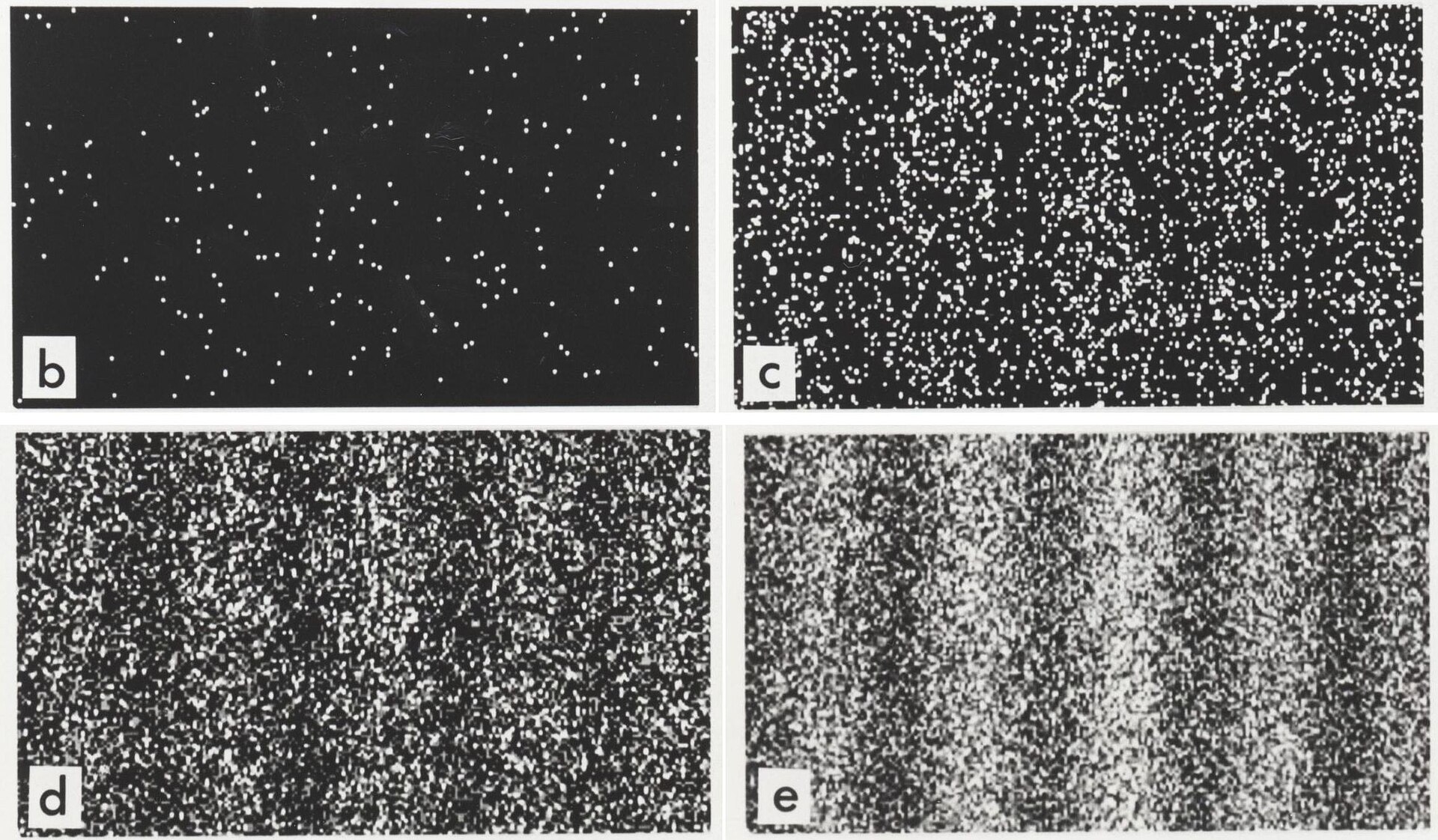
Un qubit reale, 4000 «elettroni» e la statistica di ciò che non si può prevedere

Che cosa succede se si prova a prevedere dove atterrerà il prossimo «elettrone» di una frangia di interferenza, usando come sorgente un vero computer quantistico? Abbiamo messo alla prova l’idea su hardware reale, con 17 qubit superconduttori, e il risultato più interessante non riguarda la frangia: riguarda un piccolo bias della macchina che si è fatto notare nei numeri.

Come è fatto l’esperimento

L’esperimento ha due parti. Nella prima, un circuito a un solo qubit si comporta come un interferometro a due cammini: una rotazione Ry fa da «beamsplitter», una rotazione Rz codifica la differenza di fase (l’equivalente di una differenza di cammino ottico) e una porta H ricombina i due cammini. Il circuito viene eseguito una volta per ciascuna di 21 posizioni x comprese tra −1 e +1, e la probabilità di misurare lo stato |1⟩ è letta direttamente dai conteggi dell’hardware, non calcolata a tavolino.

Nella seconda parte un circuito ancora più semplice, fatto solo di porte H seguite da misura, produce bit casuali genuinamente quantistici. Quei bit vengono trasformati, con il campionamento a trasformata inversa, in 4000 posizioni continue sulla densità interpolata dai 21 punti della prima parte. Un predittore basato su stima di densità a kernel (KDE) osserva la sequenza elettrone dopo elettrone e cerca di stimare dove cadrà il successivo, usando solo il passato.

Le domande erano due: le misure quantistiche successive sono davvero prive di «memoria»? E quanto può avvicinarsi un modello statistico al limite teorico, quello di un oracolo che conosce la distribuzione vera?

La distribuzione misurata sul chip

Istogramma della distribuzione misurata su 21 punti con 17 qubit
La probabilità normalizzata misurata nelle 21 posizioni. Il picco dominante è in x = +0,2.
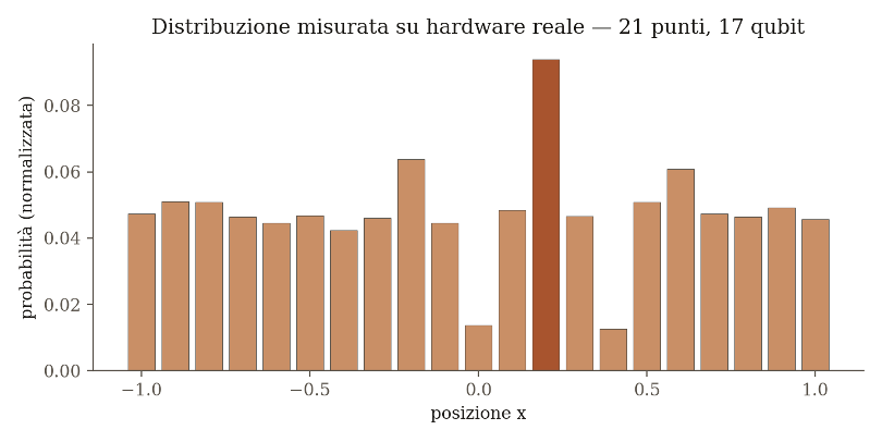
La distribuzione ha una struttura netta: un picco dominante in x = +0,2, due avvallamenti quasi nulli vicino a x = 0 e a x = +0,4, e un fondo abbastanza piatto altrove. In questa sessione non compaiono anomalie: tutti i punti stanno nell’intervallo atteso, compreso x = −0,4, che in sessioni precedenti aveva mostrato un valore anomalo. Il picco in +0,2 è stabile e riproducibile tra sessioni diverse.

4000 «elettroni» da monete quantistiche

Istogramma delle 4000 posizioni campionate con sovrapposta la densità vera interpolata
Le 4000 posizioni campionate dal computer quantistico (barre) seguono la densità interpolata dai punti della prima parte (linea).
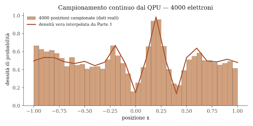
Le 4000 posizioni continue seguono visibilmente la densità della prima parte, picco compreso. Sul fronte della «memoria», l’autocorrelazione tra elettroni successivi vale 0,0125, compatibile con zero entro l’errore atteso (circa 0,016): nessuna correlazione reale tra un elettrone e il successivo.

Quanto in fretta impara il predittore

Grafico log-log del gap dall’oracolo in funzione della dimensione della finestra
Il gap dall’oracolo al crescere della finestra N (scala logaritmica) e, tratteggiato, il riferimento teorico N^(−2/5).
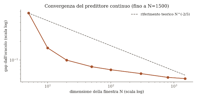
Come misura di qualità usiamo il «gap» dall’oracolo, cioè quanto la stima resta indietro rispetto a chi conosce la densità vera. Con appena 5 osservazioni il gap è 0,56; con 10 scende a 0,16, con 100 a 0,07 e con 1500 a circa 0,051. Resta sopra zero ma continua a scendere. Il fit log-log dà un esponente attorno a −0,35/−0,4, coerente con il tasso teorico dei kernel non parametrici, più lento di quello di un semplice istogramma. Per orientarsi: la log-densità dell’oracolo è −0,6458, quella di una distribuzione uniforme (il modello che non sa nulla) è −0,6931.

A che cosa serve, allora, un predittore?

Il singolo elettrone resta imprevedibile per costruzione: i campioni sono indipendenti e nemmeno l’oracolo può fare meglio dell’entropia della distribuzione. Quello che si può fare è rispondere a domande del tipo: con che probabilità il prossimo valore supererà una soglia, starà sotto un’altra, oppure cadrà tra le due? E, soprattutto, quanto ci si può fidare di quella stima.

L’incertezza si quantifica con un approccio bayesiano: con un prior uniforme, se k campioni su N cadono nella regione, la probabilità incognita ha distribuzione a posteriori Beta(k+1, N−k+1), da cui si ricava un intervallo di credibilità al 95%. Per probabilità intorno a 0,25 l’intervallo è largo circa ±2 punti percentuali con N = 1500 e circa ±1,3 con N = 4000.
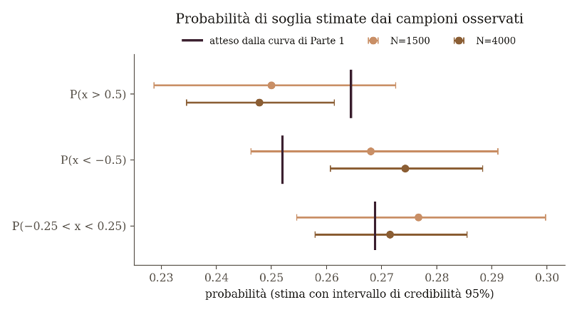
Stime di probabilità di soglia con intervalli di credibilità al 95% per N=1500 e N=4000

Tre probabilità di soglia stimate dai campioni, con intervallo di credibilità al 95%. Il segmento scuro è il valore atteso dalla curva della prima parte.

Con N = 1500 tutti e tre gli intervalli contengono il valore atteso dalla curva misurata nella prima parte. Con N = 4000 gli intervalli si stringono e due su tre lo mancano, con uno scarto sistematico: troppi campioni a sinistra (la probabilità di x < −0,5 è stimata a 0,274 contro 0,252 attesi) e troppo pochi a destra (0,248 contro 0,265 per x > 0,5). La probabilità di cadere tra −0,25 e +0,25 resta invece in linea, a circa 0,27.

Il colpevole: monete non del tutto equilibrate

Se le posizioni seguissero esattamente la curva della prima parte, la loro trasformata probabilistica u = F(x) sarebbe uniforme tra 0 e 1. Nell’ultima sessione la media di u è 0,4868 contro un valore atteso di 0,5000 ± 0,0046, e il test di Kolmogorov-Smirnov dà p ≈ 0,008: la deviazione è statisticamente significativa.
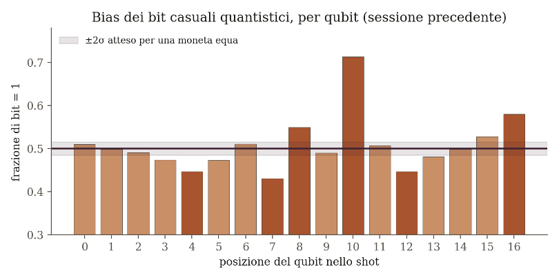
Frazione di bit pari a 1 per ciascuno dei 17 qubit, con banda di ±2 sigma

Frazione di bit pari a 1 per ogni posizione del qubit nello shot (sessione precedente). La banda indica ±2σ atteso per una moneta equa.

La spiegazione più plausibile è che i bit casuali quantistici, generati con una porta H seguita da misura, non siano equiprobabili. In una sessione precedente, di cui abbiamo i bit grezzi, la frazione di 1 varia da qubit a qubit tra 0,43 e 0,71, quando per una moneta equa ci si aspetterebbe 0,50 ± 0,008. Per l’ultima sessione i bit grezzi non sono disponibili, quindi lì la spiegazione resta un’inferenza.

Per prevedere il comportamento di questa macchina, dunque, le stime empiriche restano il riferimento giusto: descrivono la sorgente reale, bias compreso, e si discostano di circa 1-2 punti percentuali dalla curva ideale. Non è un errore del predittore, è un’informazione sull’hardware. Con due limiti: le stime valgono per la sessione e la calibrazione in cui sono state raccolte, perché l’hardware deriva nel tempo; e l’indipendenza tra elettroni è stata verificata solo con l’autocorrelazione a passo 1, che non esclude correlazioni residue tra qubit vicini dello stesso shot.

Che cosa dimostra, e che cosa no

L’esperimento mostra che l’indipendenza tra misure quantistiche successive, un postulato della meccanica quantistica standard, si può verificare empiricamente su hardware reale in modo ripetibile. Mostra anche, su dati reali e non simulati, alcune proprietà genuine della stima statistica: la diversa velocità di convergenza tra stimatori parametrici e non parametrici, il compromesso tra bias e varianza a finestre intermedie e la necessità di correzioni quando si stima una densità su un dominio limitato.

Non è invece una replica dell’esperimento di Tonomura. Lui faceva diffrangere elettroni fisici attraverso un biprisma elettronico, nello spazio reale. Qui Tonomura è stata soltanto l’ispirazione per la geometria del circuito, scelta per assomigliare a una frangia con inviluppo, ma la grandezza misurata è la statistica di un singolo qubit superconduttore. È un’analogia formale, non la stessa fisica.

E adesso: Gaussiana o Cauchy?

Per il prossimo passo ci sono due candidate. La gaussiana troncata su [−1, 1] sarebbe un caso di controllo pulito: liscia e nota analiticamente, permetterebbe di verificare se esponente di convergenza e correzione di bordo si comportano come da manuale, senza le complicazioni del picco netto e dei pozzi della frangia attuale.

La Cauchy è metodologicamente più interessante, perché è uno stress test di un punto debole noto: ha code pesanti e varianza non definita, mentre la regola con cui si sceglie la larghezza del kernel presuppone una forma vicina alla gaussiana. Servirebbe capire dove e come l’approccio attuale smette di funzionare. Resta da decidere se troncare la distribuzione, perdendo però proprio le code pesanti che la rendono interessante, o ridisegnare il dominio.

Spotting the Flaw: A Quantum-Classical Experiment in Visual Anomaly Detection

Every bottling line eventually produces a bottle it shouldn’t: a hairline fracture, a chip along the rim, a smear of contamination on the glass. Catching such defects automatically is a deceptively hard problem, not because the flaws themselves are complex, but because they are rare. A line can run for hours before producing a single bad unit, so there is rarely enough labeled defect data to train an ordinary classifier the way one might train a model to tell cats from dogs. The more practical framing, used in a recent study by the engineering team, is one-class learning: show a model thousands of images of what “good” looks like, and ask it to flag anything that deviates from that picture, without ever showing it an actual defect during training.

The study set out to compare two very different ways of drawing that boundary: a classical ensemble method called Isolation Forest, and a quantum circuit known as a Variational Quantum Classifier (VQC). Both were tested on the bottle category of MVTec AD, a widely used industrial benchmark whose images are either defect-free or flawed in one of three ways — broken_large (major structural fractures), broken_small (minor chips and cracks), or contamination (surface stains and deposits).

A shared starting point

To keep the comparison fair, both branches share an identical front end. Each 900×900 pixel image passes through a convolutional network pretrained on ImageNet with its final classification layer removed, producing not a label but a 2048-number fingerprint of the image’s visual texture and structure. Those numbers are standardized using statistics from the training set of good bottles only, so no information about the defects leaks into preprocessing, then compressed to just 10 dimensions with principal component analysis. Despite that aggressive compression, the ten retained components capture roughly half of the total variance in the embeddings — enough, it turns out, to separate the two classes; the first three components alone account for more than a quarter of it. Because both branches inherit these same ten numbers, any difference in performance downstream comes from how each classifier reasons over them, not from how the features were extracted.

Branch one: an old, reliable idea

The classical branch relies on Isolation Forest, which identifies outliers through a simple insight: anomalies are easier to isolate than normal points. The algorithm builds an ensemble of trees that split the data along random feature thresholds, and a point that differs from the bulk of the data tends to need far fewer splits before it sits alone in its own partition. This implementation used 400 such trees, fit exclusively on the compressed embeddings of defect-free bottles, and reached 91.6 percent accuracy on the test set, with a strong 98.3 percent precision on the anomaly class — it rarely cried wolf. Its weakness showed up in recall: it missed six defective bottles, mostly small chips and low-contrast contamination sitting close enough to normal texture variation to slip past the boundary.

Branch two: encoding a bottle into ten qubits

The quantum branch takes the same ten PCA values and uses each as a rotation angle, applying a Ry gate to initialize one qubit per feature. This “angle embedding” turns a classical vector into a quantum state living in a 1,024-dimensional Hilbert space, since ten qubits span two-to-the-tenth possible basis states. From there, the circuit applies three Strongly Entangling Layers: each one rotates every qubit through a further sequence of parameterized gates, then links neighboring qubits in a ring using CNOT gates, so the state of each qubit becomes correlated with its neighbor’s.

The full circuit has 90 trainable parameters, tuned with the Adam optimizer over 80 epochs, again using only defect-free images. Training pushes good bottles toward a state where all ten qubits are measured as zero; a bottle’s anomaly score is then one minus that measured probability, with the cutoff set at the 90th percentile of scores observed during training, 0.9972. The appeal of this design, in theory, is that entanglement lets the circuit represent joint, nonlinear relationships between the ten features that a tree-based model doesn’t naturally capture — though whether that theoretical appeal shows up in practice is the actual question the experiment set out to answer.

What the numbers say

The quantum circuit edged out the classical baseline, reaching 92.8 percent accuracy against 91.6, with recall improving to 93.7 percent from 90.5 — three additional defects caught, by the team’s count. It gave up a little precision in exchange, 96.7 percent versus the Isolation Forest’s 98.3, tripped up by two good bottles that scored between 0.998 and 0.999, just over the line. The quantum scores overall were sharply polarized: the great majority of defective bottles scored almost exactly 1.000, while good bottles spread more broadly across lower values, which suggests the cutoff is a reasonably stable one rather than a lucky draw. Both models, notably, stumbled on the same kind of case — subtle, low-contrast defects that resemble normal surface texture — which hints that the bottleneck may sit upstream, in the shared feature extraction, rather than in either classifier.

It’s worth being precise about what this result does and doesn’t show. The VQC here ran as a simulation on classical hardware, not on an actual quantum processor, and training it took on the order of ten to a hundred times longer than fitting the Isolation Forest, since every gradient step requires simulating a ten-qubit state vector. A recall gain at that computational cost is an interesting empirical result on one specific dataset, not evidence of a general “quantum advantage.” Both classifiers also share the same structural limits: neither can point to where on the bottle a flaw sits, since both output a single score rather than a localized map, and both thresholds are only as trustworthy as how well the training set of good bottles represents real-world variation.

The more useful reading is as a well-controlled feasibility check: a modestly sized quantum circuit can match, and here slightly exceed, a strong and far cheaper classical baseline on a real industrial vision task. The natural next steps — running the same circuit on actual quantum hardware such as IBM’s or IonQ’s processors, blending its score with a classical reconstruction-error signal, and adding tools like Grad-CAM to localize defects rather than merely flag them — should show whether this early edge survives outside of simulation, and whether it is worth the bill.

Bell inequality on real quantum hardware

Image: CERN – https://home.cern/news/news/physics/fifty-years-bells-theorem

We run a Bell test in the CHSH formulation on two real quantum platforms: the goal was not to demonstrate anything new, but to use a well-known experiment as a direct physical benchmark to understand how much a real quantum processor can preserve entangled correlations. This test could fit the purpose because it produces a number that is easy to interpret, that is the Bell parameter: if the value remains less than or equal to 2, the result is compatible with a local classical description. If it exceeds 2, a violation of Bell’s inequality is observed, and, in particular, the theoretical quantum maximum is 2*√2​, approximately 2.82843. An important aspect of this experiment is that the measurement basis is chosen using block randomization, that is instead of first measuring all the data for one given configuration and then moving on to the next, the different measurement settings are randomly mixed throughout the execution. This has been done to reduce the imperfection of the real hardware due to calibrations, noise, temporal drift, and operating conditions, thus making a random choice of measurement basis would reduce the risk. Further, this point wanted to reproduce the spirit of Alain Aspect’s experiments on the violation of Bell inequalities. In that case, the choice of measurement basis was critical: changing the orientation of the analyzers during the experiment served to avoid the particles from being interpreted as already “prepared” with respect to a fixed measurement configuration. In Aspect’s case, the change of basis therefore had a very deep foundational meaning, connected to locality and the separation between measurement choices.

In our case, much more humbly, no locality loophole is being closed: the qubits are on the same device, the experiment is digitally programmed, and the measurements are not spatially separated as in an optical Bell test and the methodological idea is: not allowing a fixed measurement configuration to dominate an ordered part of the experiment.

For each experiment, 100,000 shots were used because the quantities observed in the Bell test are derived from measured probabilities and increasing the number of shots reduces the statistical error on the observed frequencies and as a consequence on the calculated correlations.

The result (Bell parameter) on the first real hardware technology was 2.45294 ± 0.00499, well above the classical limit of 2. The deviation from the ideal quantum value was 0.37549, corresponding to about 86.7% of the theoretical maximum, that is the apparent loss of visibility was about 13.3% and the statistical significance with respect to the classical limit was approximately 90.7 sigma.

On the second real hardware technology, the result was also clearly quantum, as the measured value was 2.40736 ± 0.00505, still above the classical limit and this time the deviation from the ideal value was 0.42107, corresponding to about 85.1% of the theoretical maximum with an apparent loss of visibility of about 14.9%, with a statistical significance of approximately 80.7 sigma with respect to the classical limit.

It is useful to interpret the deviation from the ideal value not as a pure measure of a single type of “noise” but as an aggregate indicator of experimental degradation: gate errors, readout errors, decoherence, drift, and calibration imperfections all contribute to reducing the observed value, giving a better view of what measured experimentally with random circuits in previous pieces of work. In particular, it should be noted that the closer the result is to the ideal maximum, the better the device is preserving quantum correlations; the closer it moves toward the classical limit, the more noise has degraded the experiment.

Here below a sample of the used circuits and result of the 100000 runs on the first real hardware.

RESULTS ON REAL HARDWARE

E(a,b) = 0.62446 ± 0.00247 N = 100000
E(a,b’) = 0.59396 ± 0.00254 N = 100000
E(a’,b) = 0.60250 ± 0.00252 N = 100000
E(a’,b’) = -0.63202 ± 0.00245 N = 100000

S CHSH = 2.45294 ± 0.00499

Predicting Quantum Circuit Noise Sensitivity from Structure,

Entropy, and Effective Noise Scaling


Understanding how noise propagates through quantum circuits is a central problem in near-term quantum computing. While gate error rates and circuit depth provide partial explanations of circuit degradation, the relationship between circuit structure, state properties, and observable noise sensitivity remains poorly characterized. In this work we introduce a predictive framework for estimating local noise sensitivity in quantum circuits. We combine (i) an effective noise accumulation coordinate derived from gate counting, (ii) entropy-based descriptors of local state mixing, and (iii) machine learning models trained on circuit structural features. Using simulations on QASMBench circuits under depolarizing and readout noise, we show that a simple exponential saturation model based on an effective noise coordinate explains moderate variance in local total variation distance (TVD).

Keywords: quantum circuit noise sensitivity, effective noise scaling, entropy-based descriptors, total variation distance, machine learning prediction

Local Entropy as a Universal Predictor of Noise Sensitivity

in Variational Quantum Circuits


Noise accumulation limits the performance of variational quantum circuits in the noisy intermediate-scale quantum (NISQ) regime. Standard analyses typically rely on global distributional metrics, such as total variation distance (TVD) over full measurement outputs. However, in highly expressive or scrambling circuits, global TVD often saturates and becomes insensitive to structural differences between ansatz families. In this work we show that local entropy provides a universal control parameter for local noise sensitivity under depolarizing noise. We prove that the marginal TVD of one-qubit and two-qubit subsystems is upper-bounded by a function of the entropic deficit from maximal mixing. We then demonstrate numerically that scrambling circuits exhibit entropic self-averaging, leading to a universal collapse of local TVD when plotted against mean single-qubit entropy. Furthermore, we identify the ratio between two-local and one-local sensitivities as a structural marker of scrambling dynamics. These results establish local entropy as a principled and architecture-independent predictor of measurement-level noise response.

Keywords: local entropy, noise sensitivity, variational quantum circuits, depolarizing noise, marginal total variation distance


Inversion and Reconstruction of Quantum States under Continuous – Weak Measurement and Discrete Circuit Noise


Abstract

Quantum information processing is fundamentally constrained by measurement backaction and environmental noise. This work develops a unified quantitative study of quantum state degradation and reconstruction across two complementary dynamical regimes: continuous weak measurement described by stochastic master equations (SME), and discrete gate-based quantum circuits subject to depolarizing and readout noise.

In the continuous regime, we demonstrate stable exponential convergence of a stochastic quantum filter toward the true conditional state under finite detection efficiency. In the circuit regime, we analyze a bounded subset of QASMBench OpenQASM circuits under a structured noise sweep and measure output distributional divergence using Total Variation Distance (TVD). We identify an empirical exponential saturation law and show that degradation collapses onto a compact effective interaction variable.

Keywords: quantum state reconstruction, stochastic master equation, continuous weak measurement, quantum circuit noise, total variation distance, exponential scaling law


Predicting Quantum Hardware Noise from Circuit Structure

A machine learning model was developed to predict the discrepancy between ideal and experimentally measured quantum circuit output distributions when executing circuits on a real quantum hardware backend. The target quantity is the total variation distance (TVD) between the ideal distribution obtained from classical simulation and the distribution observed from hardware execution. The goal is to determine whether structural properties of a circuit, together with information derived from ideal simulation, can be used to estimate how strongly hardware noise will distort the circuit’s output.

The dataset consists of families of parameterized quantum circuits with varying depth, entangling structure, and topology. For each circuit, the ideal output distribution is computed using a classical simulator, while the same circuit is executed on a real quantum processing backend to obtain the measured output distribution. From these circuits, features describing the circuit structure (such as depth and two-qubit gate structure) and statistics of the ideal output distribution are extracted and used as inputs to a regression model.

A ML algorithm trained on these features achieves strong predictive performance when evaluated on a held-out test set drawn from the same circuit family distribution, achieving an R2 score of approximately 0.57 with a mean absolute error of about 0.033 TVD units. The model also shows a strong rank correlation (Spearman ρ≈0.82), indicating that it can reliably order circuits from more to less noise-sensitive even when exact prediction errors remain.

To test generalization beyond the training distribution, an additional experiment was conducted in which the model was trained on circuits belonging to two circuit topology families and evaluated on circuits from a third, previously unseen topology. Under this topology shift, predictive performance decreases to R2≈0.19 with a mean absolute error of approximately 0.048 and a rank correlation of ρ≈0.66. Although absolute prediction accuracy drops under this distribution shift, the model still preserves moderate ability to rank circuits by expected deviation from ideal behavior.

Overall, these results suggest that circuit-level structural features combined with ideal-simulation statistics contain meaningful information about hardware noise sensitivity. While accurate regression across unseen circuit families remains challenging, the model demonstrates promising capability for estimating relative circuit robustness prior to execution on quantum hardware that is extremely useful for high intensive and expensive workloads.